
Downloads
Download a PDF of the report here
PDF | 732.49 KB
Key findings
- Forecasts for government borrowing are uncertain and subject to frequent revision. Over the last four decades, borrowing has turned out higher than the median forecast for that year on three-quarters of occasions. In other words, forecasts have tended to underestimate the future level of borrowing. This was particularly the case just prior to periods of economic distress, such as the early 1990s, late 2000s and the pandemic, but is true generally.
- Forecast revisions often reflect economic ‘news’ since the previous forecast and unfortunately, since 2010, there has been more bad news than good. Across the 26 fiscal events since 2010, there have been just 8 occasions on which economic news has meaningfully improved the borrowing outlook, versus 12 where bad news has materially worsened the outlook. On 6 occasions, there was no meaningful change.
- Chancellors often adjust their tax and spending plans in response to these forecast changes. For example, if the economic and fiscal outlook improves, it could be that the Chancellor is able to lower taxes and/or increase spending and still be on track to meet his or her stated objectives for borrowing or debt. Conversely, if the outlook deteriorates, the Chancellor might decide to raise taxes and/or cut spending to return forecast borrowing back towards the desired level.
- It matters whether or not Chancellors respond symmetrically to good and bad news. If Chancellors respond asymmetrically to underlying changes in borrowing forecasts – for example, by spending windfall gains in the case of good news, but accommodating increased borrowing when bad news comes along – then over time, borrowing will systematically diverge from that forecast. This represents a non-trivial risk to the accuracy of borrowing forecasts, and potentially to fiscal sustainability.
- Chancellors have not responded symmetrically to good and bad economic news since 2010. On the 12 occasions when economic conditions deteriorated meaningfully between fiscal events, Chancellors have planned to offset just over a quarter (27%) of the medium-term borrowing increase, on average, by reducing the planned level of spending and/or announcing tax rises for implementation by the final year of the forecast period. Meanwhile, when economic conditions improved, Chancellors have planned to offset an average of 60% of the windfall through higher spending and/or lower taxes.
- This tendency for Chancellors to loosen more than they tighten in response to economic news led to tens, and possibly hundreds, of billions of additional borrowing over the 2010s. Public sector net debt at the eve of the pandemic could have been between 3% and 11% of GDP lower – with a central estimate of 7% – had Chancellors responded symmetrically to underlying forecast changes over the preceding decade.
- Asymmetric policy responses mean that the Office for Budget Responsibility (OBR)’s central forecast is not actually ‘central’. Based on Chancellors’ past responses to shocks, and assuming good shocks are as likely to come along as bad ones, we estimate that forecastgovernment borrowing in 2027–28 should be 1.4% of GDP higher than under the OBR’s central forecast. In 100,000 simulations of future shocks and subsequent policy responses, we estimate that there is just a one-in-ten chance that borrowing turns out lower than the OBR forecast. This is symptomatic of a wider issue facing the OBR: the requirement to take government policy as stated, rather than exercise its judgement based on past government behaviour, can make it more likely that the forecast underestimates borrowing.
- When economic conditions improve, Chancellors since 2010 have tended to top up their spending plans, rather than use any ‘windfall’ to cut taxes. When conditions worsen, they have tended to cut back their spending plans and raise taxes. Combined, this tendency has acted to increase the size of the state over time. We estimate that if future Chancellors respond to economic news in the same way as their predecessors, the forecast for total government spending should be 1.6% of GDP higher in 2027–28 than under the OBR’s central forecast. In contrast, forecast government revenues would be just 0.2% of GDP higher in our simulations.
- In the short term, Chancellors tend to announce a policy loosening (i.e. higher spending and/or lower taxes) regardless of whether there has been an underlying economic improvement or deterioration. This may be appropriate – depending on the nature of the economic news – but risks a further ‘ratcheting’ effect if short-term loosenings are implemented but medium-term tightenings are ever-postponed.
5.1. Introduction
Governments make policy choices on the basis of forecasts. This is particularly true of fiscal policy, where governments often target borrowing or debt at some future date. These forecasts are subject to considerable uncertainty, however, and are subject to frequent revisions – especially when the economy gets buffeted by shocks.
This is illustrated in Figure 5.1, which shows the range of forecasts for public sector net borrowing (PSNB) made for each year since 1982–83. In periods of unexpected economic turmoil, the range of forecasts is particularly wide. For the 2009–10 financial year, for example, the level of forecast borrowing ranged from 1.5% of GDP (in the March 2005 Budget) to 12.6% of GDP (in the December 2009 Pre-Budget Report); in the event, borrowing amounted to 10.2% of GDP. Even in less turbulent times, forecasts can still be revised by a per cent or more of GDP: the average forecast error over the past 40 years was 1.8% of GDP.1
Figure 5.1. Public sector net borrowing forecasts and out-turn since 1982
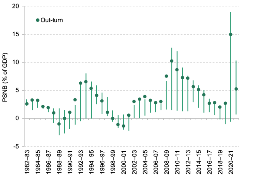
Note: Each line represents the range between the highest and lowest forecast for PSNB. From 1982–83, there are at least five forecasts for each fiscal year. Forecasts produced prior to 2010 were made by the Treasury. Out-turn data are the latest available data published in March 2023.
Source: Office for Budget Responsibility, ‘Historical official forecasts database’, https://obr.uk/data/; authors’ calculations.
Figure 5.1 also shows that borrowing tends to come in towards the top end of the forecast range. In other words, there is a tendency for most borrowing forecasts to be overly optimistic. Since 1982–83, borrowing has turned out higher than the median forecast on three-quarters of occasions. The early 1990s, the 2000s and the 2010s stand out as periods during which forecasts were particularly optimistic. The tendency for forecasts made during the 2010s to underestimate borrowing, and subsequently to be revised upwards, is illustrated in Figure 5.2.2
Figure 5.2. Successive Office for Budget Responsibility borrowing forecasts since 2009–10 and the subsequent out-turn
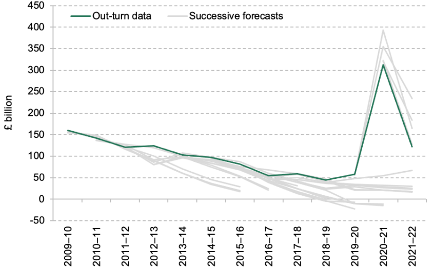
Source: Chart 1.2 of Atkins and Lanskey (2023).
As Chancellors prepare ahead of each fiscal event, they are provided with a new set of forecasts, which contain information about how the outlook has changed since the last fiscal event. These changes can be thought of representing ‘good’ or ‘bad’ economic news. Chancellors often adjust their tax and spending plans in response to this news. For example, if the economic and fiscal outlook improves, it could be that the Chancellor is able to lower taxes and/or increase spending and still be on track to meet his or her stated objectives for borrowing or debt. Conversely, if an adverse event occurs and the outlook deteriorates, the Chancellor might choose to raise taxes and/or cut spending to get (the forecast level of) borrowing back towards his or her desired level.
It matters whether or not Chancellors respond symmetrically to good and bad news. If Chancellors respond asymmetrically to underlying changes in borrowing forecasts – for example, by spending windfall gains in the case of good news, but allowing borrowing to increase when bad news comes along – then over time, borrowing will systematically diverge from the forecast.3 This represents a non-trivial risk to the accuracy of OBR borrowing forecasts, and potentially to fiscal sustainability.
A particularly blatant example of this pattern of asymmetric behaviour – previously highlighted in the 2018 IFS Green Budget – came during Philip Hammond’s period as Chancellor. His statements indicated that he would view forecast improvements and deteriorations rather differently.
In the Autumn 2017 Budget, he cited a ‘balanced approach’ when responding to a deterioration in the forecast:
‘I reaffirm our pledge of fiscal responsibility and our commitment to the fiscal rules I set out last Autumn. But now I choose to use some of the headroom I established then. So that as well as reducing debt, we can also invest in Britain’s future. Support our key public services. Keep taxes low. And provide a little help to families and businesses under pressure.’
Philip Hammond’s Autumn Budget speech, November 2017
That is, he said that he would allow borrowing to rise following a forecast deterioration (‘use some of the headroom’). Then, in the following Spring Statement (2018), he said:
‘And if, in the Autumn, the public finances continue to reflect the improvements that today’s report hints at, then, in accordance with our balanced approach, and using the flexibility provided by the fiscal rules, I would have capacity to enable further increases in public spending and investment in the years ahead.’
Philip Hammond’s Spring Statement speech, March 2018
In other words, he indicated that if the outlook for the public finances improved, he would be minded to spend any such improvement. So, in one instance, the Chancellor is saying that he will allow borrowing to increase following a forecast deterioration, rather than offset the increase through policy measures. Yet in the subsequent instance, he is promising to spend the windfall should the public finances improve. In this chapter, we examine how successive Conservative Chancellors have reacted to underlying changes in public sector net borrowing forecasts since 2010. We begin in Section 5.2 by documenting those underlying changes and defining what we mean by good and bad economic news.4
Next, we document the discretionary policy responses implemented by Chancellors over the last 13 years (Section 5.3). In Section 5.4, we then match the policy responses to the underlying changes to examine the relationship between the two.
We show that this relationship is asymmetric, in that Chancellors respond differently to good and bad news. In Section 5.5, we consider the possible implications for the OBR’s forecasts for borrowing and the size of the state over time. Section 5.6 concludes.
5.2. Changes to public finance forecasts since 2010
Since 2010, the Office for Budget Responsibility has published independent forecasts of fiscal aggregates, such as receipts and spending. They are produced and shared with HM Treasury ahead of each fiscal event, making them a key input into government decision-making.
Our focus in this chapter is on forecasts for public sector net borrowing as a percentage of GDP. A limit on borrowing is one of the government’s current fiscal targets, and it is a salient measure of the overall tightness of fiscal policy.
Importantly, at each fiscal event, in addition to providing new forecasts for borrowing, the OBR publishes data on revisions made to past forecasts. These forecast revisions are decomposed into underlying changes (see Box 5.1), policy changes announced since the forecast was made (see Box 5.2 later) and statistical classification changes. We use changes to the underlying borrowing forecast (i.e. those not caused by classification changes or subsequent policy changes) as a proxy measure for the shocks hitting the economy. If, for instance, the labour market was performing unexpectedly strongly (e.g. with a greater number of people in work than expected), that would, all else being equal, lead to higher tax receipts and a reduction in the forecast level of borrowing.
--------------------------
Box 5.1. Underlying changes: definitions and examples
According to the OBR’s definition, ‘underlying changes’ include revisions to its economic forecasts, and judgements about how the public finances will perform in a given state of the economy. They can also include the effect of changes in out-turn data and changes to the amount policy measures announced at previous fiscal events are expected to cost or yield.
Figure 5.3 provides two examples of an underlying forecast revision – one of an underlying deterioration and the other of an underlying improvement. It shows how, under the latest economic assumptions, borrowing would evolve absent any new policy measures being introduced.
Figure 5.3. What is an underlying change in public sector net borrowing?
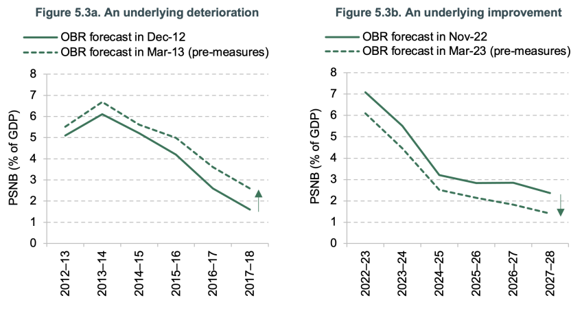
Note: The figure on the left-hand side (right-hand side) is an example of an underlying deterioration (improvement). A medium-term shock is classified as an improvement or deterioration based on the size of the final-year pre-measures forecast change relative to the previous OBR forecast.
Source: Office for Budget Responsibility, ‘Forecast revisions database’, https://obr.uk/data/; authors’ calculations.
In March 2013, underlying conditions increased the borrowing outlook relative to the December 2012 Autumn Statement (Figure 5.3a). This raised the pre-measures forecast for 2017–18 (the final year of the forecast) by 1.0% of GDP from 1.6% of GDP to 2.6%.
In contrast, the latest OBR forecast (March 2023) shows an underlying improvement (Figure 5.3b). By 2027–28 (the final year of this forecast), prior to any new policy measures, PSNB was forecast in March 2023 to be 1.0% of GDP lower than in the previous November 2022 forecast (1.4% of GDP versus 2.4%).
--------------------------
We focus solely on documenting the policy responses to medium-term shocks – that is, underlying changes to the level of borrowing in the final year of the forecast horizon.5 These changes may either increase the borrowing outlook as a percentage of GDP (a ‘deterioration’, or ‘bad news’) or decrease it (an ‘improvement’, or ‘good news’).
There may also be no news: since 2010, there have been six fiscal events when the final-year change was small – between –0.25% and +0.25% of GDP – which we classify as meaning there was ‘no change’ in the borrowing outlook (Figure 5.4).
Figure 5.4. Underlying medium-term changes by fiscal event
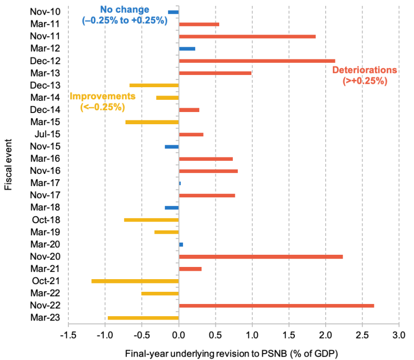
Note: All values denote the underlying change in the final year of the forecast period. November 2020 combines the forecast revisions made in the Fiscal Sustainability Report and Summer Economic Updates, as well as those in the November 2020 fiscal event.
Source: Office for Budget Responsibility, ‘Forecast revisions database’, https://obr.uk/data/; authors’ calculations.
Across the 26 fiscal events since 2010, then, the government has faced 20 sizeable medium-term shocks. There have been somewhat more deteriorations (12) than improvements (8). These deteriorations have also, on average, been larger (+1.1% of GDP) than improvements (–0.7% of GDP). Across those 20 fiscal events, the mean underlying change was a 0.4% of GDP increase in borrowing. Across all 26 fiscal events (i.e. including those with no material change), the mean underlying change was 0.3% of GDP and the total sum of all underlying changes since 2010 amounts to an 8.0% of GDP increase in the final-year borrowing forecast. In other words, there has been more bad than good economic news since 2010.
The largest negative shock occurred in November 2022, following a sharp increase in energy prices and interest rates.6 The largest positive shock occurred in October 2021, during the turbulent and highly uncertain COVID period. To avoid our results being influenced by the uncharacteristic nature of both shocks and policy responses during the pandemic, we exclude the November 2020, March 2021 and October 2021 fiscal events from our main analysis.7
These shocks to the public finances are typically driven by changes in receipts rather than changes in spending (see ‘Automatic stabilisers and underlying changes’ in the appendix). This is true regardless of whether the change is an underlying improvement or deterioration. This result is not particularly surprising: large chunks of government spending are fixed in cash terms (such as public service budgets) and/or are relatively invariable to the state of the economy (e.g. spending on the state pension), whereas tax revenues are typically more cyclical. It suggests that our measure of ‘economic news’ is indeed capturing changes to the (forecast) state of the economy.
5.3. Discretionary policy announcements by fiscal event
Chancellors – or at least Chancellors who make it to a fiscal event with a new set of OBR forecasts – take fiscal policy decisions in light of the underlying changes we described in the previous section. These policy choices are discretionary. That is, they are made based on the judgement of policymakers and are the result of an active decision, rather than happening automatically (see Box 5.2).
--------------------------
Box 5.2. What do we mean by a discretionary policy change?
Borrowing plans can change as a result of discretionary or non-discretionary policy. The latter, often referred to as the automatic component of policy, varies as a result of developments that are largely outside of the government’s control. For example, if economic conditions deteriorate, we are likely to see reduced revenues from taxes on incomes, spending and profits. This would potentially come alongside higher unemployment and therefore more benefit claimants, causing government expenditure to rise. All of this would happen without any active decision from policymakers.
In this analysis, we focus on changes in PSNB forecasts that are the result of changes in discretionary policy. These refer to the active decisions by the government to change budgets, rates or rules in the tax system. For example, in the March 2023 Budget, the government made an active decision to expand the generosity of childcare support for working parents, and to scrap the lifetime allowance for private pension saving – all discretionary decisions. The same Budget saw an increase in forecasts for spending on disability benefits (see Chapter 4), but this reflected a steep rise in claimant numbers and was not due to a discretionary policy decision.
To isolate the effect of these discretionary government decisions on the borrowing forecast, the OBR categorises the following as a policy response, net of indirect effects:
- Scorecard measures: policy measures presented on the Treasury’s scorecard table.
- Non-scorecard measures: policy changes that the Treasury has chosen not to present in the scorecard.
- Changes to departmental expenditure limits: policy changes above and beyond the OBR’s judgement about underspending against plans or neutral switches of spending between departmental expenditure limits (DELs) and annually managed expenditure (AME) within total managed expenditure.
In Box 5.1, we provided an example of an underlying improvement in the borrowing forecast between Chancellor Jeremy Hunt’s Autumn Statement in November 2022 and his Spring Budget in March 2023. At the latter, the OBR’s pre-measures forecast for borrowing in 2027–28 was 1.4% of GDP, instead of the 2.4% previously thought – an improvement of 1.0% of national income.
In response, the government announced policies, such as the expansion of government-funded childcare, that the OBR estimated would reverse 30% of that pre-measures improvement by 2027–28 (Figure 5.5).We refer to this increase relative to the March 2023 pre-measures forecast as a policy ‘loosening’, even though it still leaves borrowing below what had been forecast in November 2022.
Figure 5.5. Example of a medium-term policy loosening: the Spring 2023 Budget
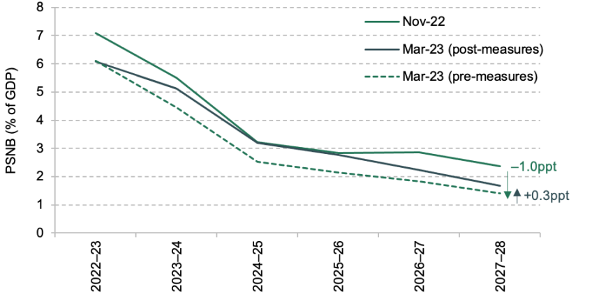
Note: Dark green (dark grey) arrows represent changes in the forecast due to underlying (policy) changes. The dark grey upward arrow reflects an announced policy loosening, while the dark green downward arrow reflects an underlying economic improvement.
Source: Office for Budget Responsibility, ‘Forecast revisions database’, https://obr.uk/data/; authors’ calculations.
--------------------------
The OBR estimates the impact of the discretionary government decisions announced at each fiscal event on its borrowing forecasts. If the policy response increases the final-year borrowing forecast relative to the pre-policy-measures forecast, policy has ‘loosened’. If it decreases it, policy is said to have ‘tightened’.
Across all 26 fiscal events since 2010, there have been as many policy tightenings as loosenings (Figure 5.6). After excluding the six fiscal events where the underlying change (or ‘shock’) has been categorised as ‘no change’, this remains the case: there have been 10 tightenings and 10 loosenings.8
Figure 5.6. Discretionary medium-term policy changes by fiscal event
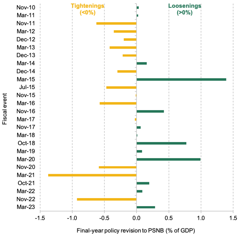
Note: All values denote the impact of policy announcements in the final year of the forecast period (and so do not include policy measures that only have short-term impacts, such as the emergency pandemic measures announced in 2020). Green bars represent a policy loosening, i.e. the government has increased borrowing relative to the pre-measures forecast. Yellow bars denote a policy tightening relative to the pre-measures forecast.
Source: Office for Budget Responsibility, ‘Forecast revisions database’, https://obr.uk/data/; authors’ calculations.
Taking the entire period since 2010, the average policy adjustment in absolute terms is 0.4% of GDP, about half the size of the average underlying change in absolute terms and equivalent to around £10 billion in today’s money.9 And although there were as many policy loosenings as policy tightenings, the tightenings were larger on average. As a result, the total sum of all policy adjustments since 2010 amounts to a cumulative tightening of 1.6% of GDP.10 In other words, the net impact of all policies announced since 2010 has been an overall tightening of the fiscal stance. That reflects the fact that Chancellors have had to respond to considerably more bad economic news than good news over that period. It does not, as we will show, mean that Chancellors have been inclined to tighten more than they loosen in response to unexpected news; it instead says more about the nature of the news experienced since 2010.
The largest tightening of the period was announced in March 2021 by then-Chancellor Rishi Sunak and included an increase in the main rate of corporation tax from 19% to 25% and a freeze in income tax thresholds. In fact, the tightening as we measure it here understates the eventual tax rise from this announcement, as inflation has since turned out much higher than expected and the freeze in thresholds has raised substantially more (see Chapter 4 and Waters and Wernham (2022)).
Outside of the COVID period, the largest tightening over the period since Autumn 2010 occurred in November 2022. This contained substantial cuts to planned spending beyond March 2025 and coincided with the largest deterioration in underlying conditions.11 Meanwhile, the largest loosening occurred in March 2015, just a few weeks prior to the general election of that year, when then-Chancellor George Osborne changed his spending assumption for the final year of the forecast (2019–20), which implied a £20 billion increase in spending plans for that year.
5.4. Do Chancellors respond symmetrically to good and bad shocks?
We now combine the data on changes in underlying conditions with the data on discretionary policy responses, to examine whether Chancellors respond symmetrically to good and bad news about the public finances.
Figure 5.7 plots all of the underlying changes alongside their associated policy responses, at each fiscal event over the last 13 years. It can be seen that policy loosenings tend to follow underlying improvements, and policy tightenings tend to occur after deteriorations. This is as we might expect: when economic conditions worsen, medium-term policy adjusts to offset some of the increase in borrowing, and vice versa. In 90% of cases when underlying conditions improved (a positive shock), policy was loosened; in 75% of cases when underlying conditions worsened (a negative shock), policy was tightened. Meanwhile, there is no clear association between policy responses and underlying changes in the medium term in the absence of a significant shock.
Figure 5.7. Medium-term policy response by fiscal event, 2010 to 2023
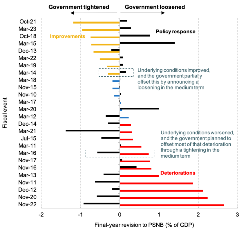
Note: Values denote the change in the final year of the forecast period. Coloured bars represent the medium-term shocks by fiscal event. Black bars represent the subsequent policy responses by fiscal event, where positive (negative) values imply a final-year forecasted tightening (loosening) relative to the pre-measures forecast.
Source: Office for Budget Responsibility, ‘Forecast revisions database’, https://obr.uk/data/; authors’ calculations.
At the top and bottom end of the figure, we have the largest improvement and deterioration, respectively. In November 2022, the government faced an underlying deterioration of 2.7% of national income in the final-year borrowing outlook. Mr Hunt subsequently announced policy to offset just over a third of the increase, or 0.9% of national income. Meanwhile, in October 2021, the government pencilled in an additional spend equal to one-sixth of the windfall gained from the underlying improvement.
While the medium-term policy response typically offsets medium-term changes in underlying conditions, short-term policy need not. Different shocks will require different immediate policy actions (e.g. in the immediate response to the pandemic). In the medium term, there is a much stronger case that policy should be symmetric and set with regard to fiscal sustainability. One concern, though, might be that Chancellors opt for short-term giveaways (appropriately or inappropriately) and at the same time promise medium-term tax rises or spending cuts which never actually come to be implemented. This phenomenon is described in Box 5.3.
--------------------------
Box 5.3. Differences over the forecast horizon
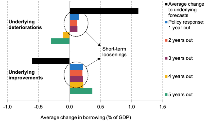
It has become common to describe UK Chancellors as behaving in the manner of St Augustine – ‘Oh Lord, give me chastity, but do not give it yet’. The decision to tighten, but not just yet, appears to describe the policy responses of Chancellors to past deteriorations well over the last 13 years. The upper panel of Figure 5.8 shows that following a deterioration in the forecast, Chancellors tend to loosen policy in the short term and tighten it in the medium term. That is, they announce higher spending and/or lower taxes in the near term but promise – promise! – to cut spending and/or raise taxes in four or five years’ time.
Figure 5.8. Average policy response in each year of the forecasting horizon
Note: Excludes fiscal events where there was no change in the underlying conditions. Negative (positive) values on the horizontal axis represent improvements (deteriorations) in the PSNB forecasts. The analysis also excludes fiscal events that occurred between November 2020 and October 2021 (inclusive).
Source: Office for Budget Responsibility, ‘Forecast revisions database’, https://obr.uk/data/; authors’ calculations.
Notably, though, Chancellors tend to loosen short-term policy regardless of whether there has been good or bad news: the lower panel of Figure 5.8 similarly shows a tendency for policy to loosen in years 1 to 3 following a forecast improvement.
The broader concern is that having announced and implemented a short-term loosening, the medium-term tightening never actually materialises – perhaps because, by that point, some other short-term shock has come along. This Augustinian behaviour would lead to more borrowing and more debt compared with a situation with full follow-through. To give one example, at the November 2017 Budget, then-Chancellor Philip Hammond announced billions of extra spending in the short term (including billions extra for the NHS and to fund preparations for Brexit), but pencilled in extremely tight spending plans for 2022–23 (the then-final year of the forecast), reducing the borrowing forecast for that year by £5 billion in the process. In the event, those plans were not stuck to: spending turned out much higher (not least because the government announced tens of billions of pounds of additional funding for the NHS in June 2018). The short-term loosening happened. The medium-term tightening did not.
The OBR’s recent analysis of its forecast performance concluded that its tendency to underestimate government borrowing derives primarily from a tendency to underestimate the medium-term level of government spending (Atkins and Lanskey, 2023). This is a manifestation of the same problem: Chancellors are prone to pencilling in very tight spending plans for the medium term, but those plans do not tend to be delivered. Instead, when it comes to a Spending Review (at which point department-by-department budgets have to be specified), spending plans tend to be revised upwards (Atkins and Lanskey, 2023).
--------------------------
Discretionary policy responses by type of forecast revision
To avoid any systematic effect on the path of the deficit, medium-term policy must respond symmetrically to medium-term shocks. One extreme case would be for Chancellors to offset entirely both good and bad shocks; another would be for them not to offset the shocks at all, and fully accommodate the increase or decrease in borrowing (which would, on average, leave borrowing unchanged over time as long as good and bad shocks were of offsetting magnitudes). In reality, Chancellors’ response functions lie between these two extremes. What matters for the presence or absence of a ‘ratcheting’ effect is whether those response functions are symmetric.
We find that, on average, around 60% of underlying improvements are offset through higher spending and/or lower taxes (a fiscal loosening), while just over a quarter (27%) of deteriorations are offset through lower spending and/or higher taxes (a fiscal tightening). If we include policy responses during the pandemic, these shares are 51% and 36%, respectively (Table 5.1).
Table 5.1. Estimated policy response functions since May 2010
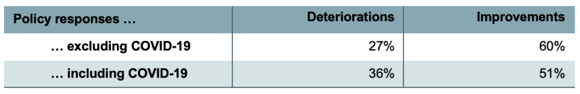
Note: Values denote the percentage of the underlying forecast change that is offset (on average) through discretionary policy changes: the ‘policy response function’. We assume the government does not respond (i.e. 0%) to underlying changes between the values of +0.25% and –0.25% of GDP, which we classify as representing ‘no change’.
Source: Office for Budget Responsibility, ‘Forecast revisions database’, https://obr.uk/data/; authors’ calculations.
The asymmetry could be caused by multiple factors. Governments may decide to take longer than five years to offset deteriorations, especially if those deteriorations are large in the short term. Deteriorations may also be harder to offset, especially politically. The key thing is that, for whatever reason, Chancellors since 2010 have systematically tended to spend a bigger fraction of forecast improvements than they have offset forecast deteriorations.
If these responses persist into the future, we can adjust our expectations about how future policy may respond to shocks and what this might mean for borrowing. Figure 5.9 maps the expected policy responses to final-year revisions to PSNB forecasts. The steeper the line, the more policy reacts to shocks. On the 45-degree line, medium-term shocks are fully offset. On the horizontal axis, medium-term shocks are fully accommodated, with no policy response.
Figure 5.9 Average policy response functions
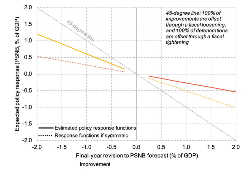
Note: Solid lines represent the estimated asymmetric policy response function. Dotted lines are perfectly symmetric versions of these estimated policy response functions. Negative (positive) values on the horizontal axis represent improvements (deteriorations) in the PSNB forecasts.
Source: Office for Budget Responsibility, ‘Forecast revisions database’, https://obr.uk/data/; authors’ calculations.
The estimated policy responses are solid lines, and perfectly symmetric versions of those responses are traced out as dotted lines. The asymmetry is clear: in the case of an improvement (left-hand side), a greater fraction of this is offset than in the case of a deterioration (right-hand side).
The tendency to spend a greater share of medium-term improvements than is offset for medium-term deteriorations will increase future borrowing relative to OBR forecasts (see Section 5.5). It will also have increased the amount the UK government has borrowed since 2010.
Recall that Chancellors since 2010 have tended to spend 60% of any improvement and offset 27% of any deterioration, on average. Over the 2010s (2010–11 to 2019–20), we estimate that had Chancellors accommodated and offset medium-term shocks in equal measure, borrowing would have been between 0.4% and 1.4% of GDP lower per year on average (with the lower figure corresponding to the case where Chancellors offset 27% of both good and bad news, and the higher figure to the case where they offset 60% of good and bad news).12 As described above, the overall impact of policy over the period was a cumulative net tightening of 1.6% of GDP, because bad shocks came along more frequently and were larger in magnitude. But had Chancellors behaved symmetrically, the net tightening would have been larger (either because of smaller loosenings in response to good news or because of larger tightenings in response to bad news).
Cumulatively, this equates to a substantial amount of additional public sector borrowing (depending on the assumptions used, between £75 billion and £260 billion extra over the course of the decade), which means a substantial amount of additional public sector debt. Figure 5.10 shows an example of a ‘symmetric’ path for borrowing (the average of the two cases above), compared with the out-turn.
Figure 5.10. An estimated path for public sector net borrowing over the 2010s with a symmetric response to shocks
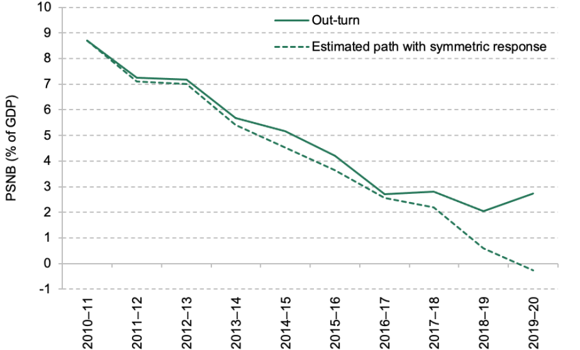
Note: The estimated path is calculated assuming symmetric policy responses to the actual shocks Chancellors have faced. When no underlying changes have occurred, we assume no policy response. During the COVID period, we use the actual policy responses. Classification changes are included. The symmetric policy response is an average of the responses if 60% and 27% of shocks are offset.
Source: Office for Budget Responsibility, ‘Forecast revisions database’, https://obr.uk/data/; authors’ calculations.
Excluding any effects on the level of debt interest costs, our estimates suggest that public sector net debt in 2019–20 might have been between 3% and 11% of GDP lower had Chancellors behaved symmetrically over the 2010s, with a central estimate that debt might have been 7% of GDP lower.13 This is not to suggest that borrowing should have been lower, or that the government should have been running a budget surplus by 2019–20 (as per Figure 5.10 or indeed as was legislated by George Osborne after the 2015 general election). It might well have been optimal to plan for looser fiscal policy in the first instance. The point is that whatever the starting point – i.e. even if the post-2010 government had set out to run looser fiscal policy – the tendency to respond asymmetrically to subsequent good and bad economic news would have led to substantial amounts – potentially hundreds of billions – of extra borrowing over the course of the decade.
Tax and spending responses
Discretionary policy responses can be decomposed into changes in spending and tax changes. On balance, discretionary changes tend to be skewed towards spending adjustments, especially after an underlying improvement (Figure 5.11). In other words, following good news, Chancellors tend to increase spending rather than cut taxes (left-hand panel). Following bad news (right-hand panel), Chancellors tend to announce a combination of spending cuts and tax rises (with more of the former than the latter).
Figure 5.11. Policy responses come predominantly through spending measures
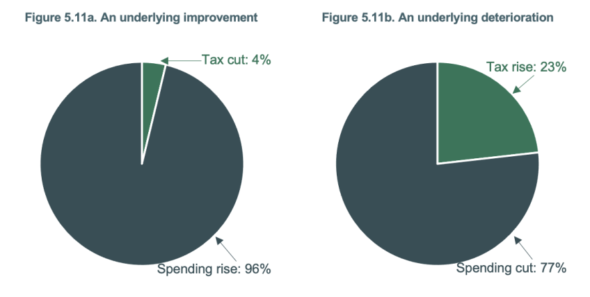
Source: Office for Budget Responsibility, ‘Forecast revisions database’, https://obr.uk/data/; authors’ calculations.
Combined, these findings suggest that Chancellors’ responses to shocks have tended to increase the size of the state. We explore this in greater detail in Section 5.5.
5.5. Implications of an asymmetric response function
Implications for borrowing forecasts
Asymmetric policy responses to underlying changes in the PSNB forecasts will alter the outlook for future borrowing. The OBR is prohibited from incorporating its own judgements about future government policy in its forecasts. For example, it has to take stated government policy on fuel duties – that rates will increase each year in line with the RPI measure of inflation – as given in its central forecast, despite the clear evidence that the government has no intention of actually increasing them. Neither can the OBR make assumptions about future asymmetric policy responses to economic news. For that reason, its central forecast is likely to underestimate the future path of borrowing.
To quantify this, we apply our policy estimates to 100,000 randomly generated medium-term economic shocks (based on the distribution of past shocks), which we assume to represent good or bad news with equal probability.14 We further assume that there continue to be two fiscal events per year, and that future Chancellors’ policy response function to shocks is the same (on average) as those of Conservative Chancellors since 2010. This exercise thus provides an indication of what borrowing could look like if Chancellors behave in future as they have in the recent past.
Figure 5.12 shows the OBR’s central forecast of PSNB, produced in March 2023.15 In addition, we plot the estimated trajectory of borrowing based on our simulations, which build in asymmetric policy responses to future shocks. Lastly, as an alternative benchmark, we include a ‘fully asymmetric’ scenario, which is an extreme case where any windfall from a forecast improvement is fully spent, while deteriorations are not offset at all.
Figure 5.12. Central borrowing forecasts under different assumptions
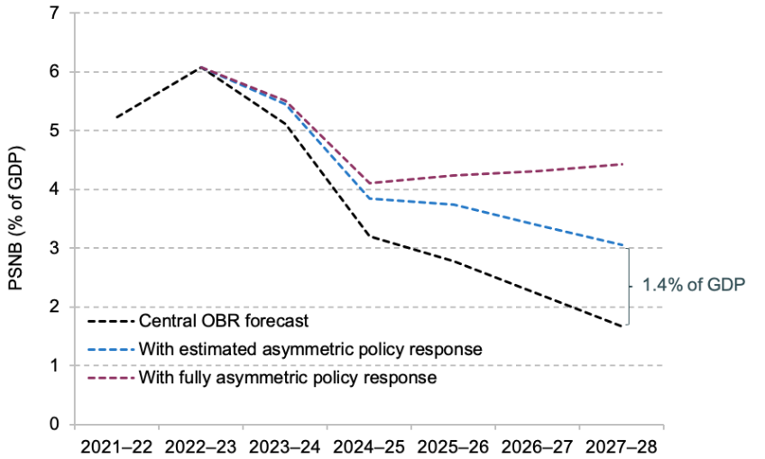
Note: Policy response series are based on 100,000 simulations of forecast errors and subsequent policy responses.
Source: Authors’ calculations using Office for Budget Responsibility, ‘Forecast revisions database’, http://obr.uk/data/.
In the fully asymmetric case (denoted by the purple dashed line), borrowing could not fall below the forecast level (as any improvement in the forecast would be fully offset by a policy loosening, while all forecast deteriorations would be accommodated through higher borrowing). We estimate that this would put borrowing on a rising path after 2024–25. In contrast, under our estimated asymmetric policy response scenario (which is based on how Chancellors have behaved since 2010, excluding the COVID-19 period), borrowing would continue to fall after 2024–25 but would remain substantially higher than the OBR’s central estimate.
The simulation exercise shows that treating public finance improvements and deteriorations differently can have a substantial impact on the path for borrowing. Our estimates, which anticipate policy responses to future shocks, would suggest that PSNB is likely to be around 1.4% of GDP higher in 2027–28 than under the OBR’s forecast – equivalent to £36 billion in today’s money.
To further highlight the importance of accounting for policy asymmetry, we plot the likelihood of actual borrowing turning out higher than the OBR’s central forecast (Figure 5.13). Under our assumptions, if future Chancellors respond to future economic news in the same way that Chancellors since 2010 have done, then PSNB would end up higher than the OBR forecast on 90% of occasions. Otherwise stated, there is only a one-in-ten chance borrowing would end up lower than forecast.
Figure 5.13. An overly optimistic borrowing outlook
Source: Authors’ calculations using Office for Budget Responsibility, ‘Forecast revisions database’, http://obr.uk/data/.
This estimate is sensitive to modelling assumptions. We assume that good and bad shocks come along with equal probability: if negative shocks occur more often, as they have done over the last 13 years, our future borrowing estimate would be even higher.
We also assume Chancellors will have two fiscal events per year to adjust policy in response to underlying changes. Previous analysis from the 2018 IFS Green Budget (Emmerson and Pope, 2018) shows a single fiscal event would restrict the impact of policy asymmetry on borrowing (by giving Chancellors fewer opportunities to behave asymmetrically), thereby lowering the PSNB outlook by approximately 0.3% of GDP relative to our two-fiscal-event projection (from 1.4% of GDP higher to 1.1% higher).16
Lastly, our estimates exclude policy responses during the pandemic, when the size and nature of shocks and policy responses were atypical. Including the pandemic period in our analysis lessens the asymmetry of Chancellors’ estimated policy response functions (see Table 5.1). Thus, by including pandemic responses, our borrowing forecast moves closer to the OBR’s central estimate reducing the gap to 1.1% of GDP (from 1.4% of GDP).
But while the precise figure is sensitive to these assumptions, the broader point is not: once we account for asymmetric policy response functions, the OBR’s ‘central’ forecast no longer seems so central.
Implications for the size of the state
Finally, we can estimate the implications for future levels of spending and tax revenues. In Section 5.4, we highlighted asymmetry not only in the policy responses, but also in the composition of those responses: Chancellors tend to increase spending following a forecast improvement, and to cut spending and raise taxes following a forecast deterioration. In Figure 5.14, we show the implications of that asymmetry for total managed expenditure (TME) and public sector current receipts (PSCR) under our ‘estimated asymmetric policy response’ scenario (Figure 5.13). We estimate that, if future Chancellors behave like their predecessors, then asymmetric policy responses will act to systematically increase the size of the state relative to forecast. By 2027–28, under our estimates, total spending would be 1.6% of GDP higher than under the OBR central forecast, and taxes would be 0.2% of GDP higher (which combine to give the 1.4% of GDP of extra borrowing in Figure 5.12).
Figure 5.14. Forecasts for the size of the state with asymmetric policy responses
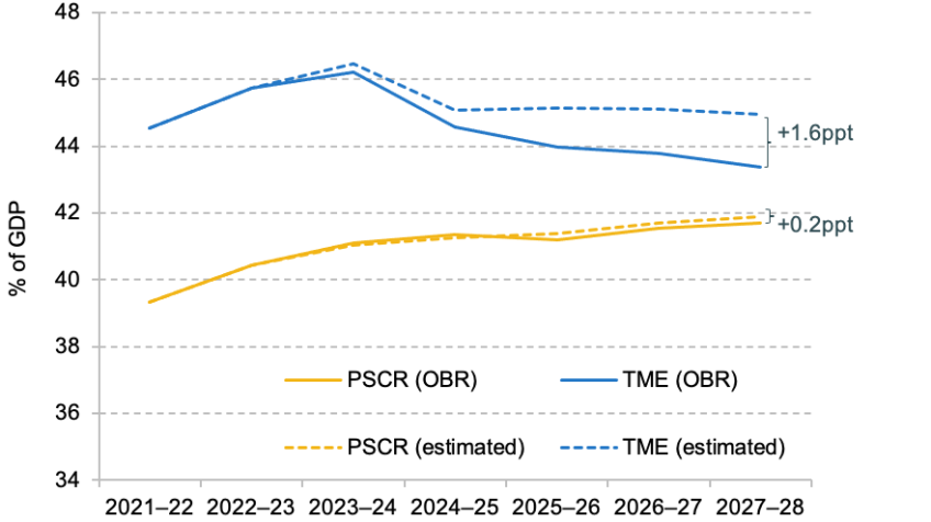
Source: Authors’ calculations using Office for Budget Responsibility, ‘Public finances databank – July 2023’, https://obr.uk/public-finances-databank-2023-24/.
5.6. Conclusion
Since 2010, there has been more bad economic news than good: things have turned out worse than expected, on average. We would expect, as a result, UK government borrowing to have turned out higher than initially planned. This has indeed been the case, as Chancellors have partly accommodated bad news by allowing borrowing to rise. The overall impact of policy over the period was a cumulative net tightening of 1.6% of GDP, because bad shocks came along more frequently and were larger in magnitude, but this offset only around one-fifth of the total increase in borrowing caused by underlying forecast deteriorations.
But part of the reason borrowing has turned out higher (over and above the impact of negative economic shocks) is that Chancellors have tended to loosen policy in response to good news to a greater extent than they have tended to tighten in response to bad news. That is, had Chancellors behaved symmetrically, the cumulative net tightening would have been even larger (either because of smaller loosenings in response to good news or because of larger tightenings in response to bad news) and the UK government would have cumulatively borrowed substantially less over the 2010s.
This is not to suggest that borrowing should have been lower over the 2010s. The point is that whatever the starting point – i.e. even if the post-2010 government had set out to run looser fiscal policy from the outset – the tendency to respond asymmetrically to good and bad economic news would have led to tens or even hundreds of billions of extra borrowing over the course of the decade.
Economic and fiscal forecasting is difficult. For the OBR – whose forecasts matter more than most, given their role in the policymaking process – it is even more difficult, as it is required by Parliament to take governments at their word and to take stated policy as given. As this chapter has demonstrated, the tendency of successive Chancellors to respond asymmetrically to economic news (an asymmetry which the OBR can point out, but cannot build into its forecasts) means that the official ‘central’ forecast cannot really be thought of as ‘central’, if future Chancellors behave anything like their predecessors. In fact, our simulations suggest that there is just a one-in-ten chance that borrowing in five years’ time turns out lower than under the OBR’s central forecast. In our central case, we estimate that government borrowing in 2027–28 will be 1.4% of GDP higher than under the OBR’s central forecast – more than enough to miss the government’s target for debt to be forecast to fall as a fraction of national income.
If Chancellors cannot credibly commit to behaving (more) symmetrically, then one option to limit the impact of their asymmetric behaviour would be to provide them with fewer opportunities to adjust policy, by having just one fiscal event per year. By providing fewer opportunities for headline-grabbing policy measures, and potentially freeing up time for longer-term strategic thinking, such a change would likely improve the quality of fiscal policymaking more generally.
Automatic stabilisers and underlying changes
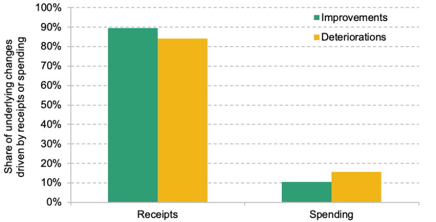
Underlying forecast changes are typically dominated by changes in receipts over changes in spending. On average, 87% of final-year underlying forecast revisions are the result of tax receipts changes. This high share holds irrespective of whether the economic news is positive or negative (Figure 5A.1).
Figure 5A.1. Underlying changes are driven by changes in receipts
Source: Office for Budget Responsibility, ‘Policy measures database’, https://obr.uk/data/; authors’ calculations.
These are average figures. There are a small number of exceptions, where underlying changes were primarily driven by spending. These include the two fiscal events either side of the 2015 general election – March and July 2015 – and March 2021, a Spring Budget at the height of the pandemic.
The tendency for underlying changes to be determined by changes in receipts is unsurprising. Tax revenues are typically more cyclical, while large proportions of government spending are, at least in the short term, invariable to the state of the economy (most obviously, departmental budgets, which are fixed in cash terms). It suggests that our measure of ‘economic news’ is indeed capturing changes to the (forecast) state of the economy.
COVID-19
The pandemic was – we hope – a once-in-a-generation event, and not a typical economic shock. The economic dislocations were of a different magnitude from anything experienced in recent memory. As well as being atypical in size, they were unusual in being (in expectation) short-term and largely temporary in nature.
The fiscal policy response was similarly atypical. In 2020–21, the government response to the public health emergency increased in-year borrowing estimates between the Spring and Autumn Budgets by 12.8% of GDP. In the period since November 2010, the next largest in-year policy change came in December 2012 (when £3.5 billion of proceeds from a 4G spectrum auction scored as negative in-year capital spending). The discretionary pandemic response, alongside deteriorating economic conditions, increased the forecast for borrowing in 2020–21 from 2.4% of GDP in March 2020 to 19.0% by November 2020.
Because the COVID-19 shock was so different in scale and nature, and because this plausibly meant a very different policy response function, we exclude the period from our main analysis. Our analysis focuses on the medium-term policy response to underlying changes in the medium-term economic outlook, and so it makes sense to abstract away from the (very different) policy responses to a low-probability short-term disruption. We do, however, test the robustness of our estimates to the inclusion of the pandemic period.
Estimating the path of PSNB under a symmetric policy response function
Since 2010, Chancellors have not responded symmetrically to improvements and deteriorations in underlying forecast revisions. Had they, the path of borrowing could have been lower since 2010 (as illustrated in Figure 5.10).
To estimate the difference between actual borrowing and an estimated version of it, we decompose borrowing changes into three parts: underlying changes, statistical classification changes and policy changes.
In our estimated ‘symmetric policy response’ scenario, we assume the same underlying and classification changes that actually occurred. However, depending on the type of underlying change – whether it was an improvement, no material change or a worsening – we replace the actual policy response with what the policy response would have been had Chancellors responded symmetrically to good and bad news (improvements and deteriorations in the underlying forecast). We assume no policy response in cases where there was no material change, i.e. where the underlying forecast change was 0.25% of GDP or less.
There are two further assumptions we introduce. The uncharacteristic nature of economic shocks and the subsequent policy responses during the pandemic means we take the actual policy responses that Rishi Sunak implemented during that time, not a symmetric version of them. We also assume that every new fiscal year entering the forecast takes the same value as estimated by the OBR. For example, the first forecast of borrowing for 2017–18 entered the OBR’s forecast period in December 2012. We take this initial value (which in this case was 1.6% of GDP) to be the starting point, to which future policy changes then apply. The analytical approach is summarised in Figure 5A.2.
Figure 5A.2. Retrospectively estimating PSNB using symmetric policy responses
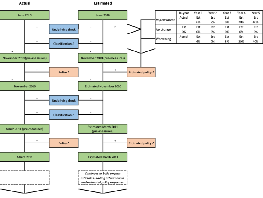
Note: Classification changes are included to get the most accurate comparison of PSNB. The only difference between the estimated PSNB figure and the actual PSNB figure is the difference between the actual policy response and the estimated (symmetric) policy response, which is a function of whether the latest shock is an improvement, no change or a worsening. When no material underlying changes have occurred, we assume no policy response. During COVID-19, we take the actual policy responses. As a new fiscal year enters the forecast, we take the actual PSNB figure expected from that year.
Simulating PSNB forecasts with asymmetric policy responses
There are three main inputs into our simulations: (i) the fraction of each final-year underlying change offset by the policy response; (ii) the rate at which the final-year underlying change permeates through the forecast horizon; and (iii) the number of fiscal events that we expect to occur over the forecast horizon.
The first input takes the ratios of the average policy responses in years 1 through to 5 to the final-year underlying change. These ratios can be calculated from Figure 5.8. The second takes the ratios of the average underlying changes in years 1 through to 5 to the final-year underlying change. These ratios are presented in Figure 5A.2. Lastly, we assume there will be two fiscal events per year over the forecast horizon.
Under these assumptions, Chancellors will set policy at 10 fiscal events between Autumn 2023 and March 2028. At each event, they will face a final-year underlying forecast revision. To get an expected policy response, we run 100,000 simulations of what has occurred over the last 13 years. That is, we assume the underlying forecast revisions and subsequent policy responses between now and 2028 will be similar in nature to those that have occurred since 2010, excluding the pandemic.
Averaging the shocks and policy responses at each of the next 10 fiscal events, we are able to build a picture of borrowing. The lines in Figures 5.12, 5.13 and 5.14 represent the mean borrowing outlook from our simulations relative to the OBR’s central estimate.
Endnotes
Authors

Carl Emmerson
Carl, a Deputy Director, is an editor of the IFS Green Budget, is expert on the UK pension system and sits on the Social Security Advisory Committee.

Isabel Stockton
Isabel works in the Healthcare sector, and on the public finances. Their research focuses on retaining and developing the NHS workforce.

Sam van de Schootbrugge

Ben Zaranko
Ben is a Senior Research Economist and an editor of the IFS Green Budget. His work focuses on the health and social care system and UK fiscal policy.
More from IFS
Understand this issue


Policy analysis


Academic research


